
Measuring proportionality

Let’s look at how we measure (dis)proportionality of elections.
What are we measuring?
We do not measure the proportionality of electoral systems per se, but the proportionality of election results. (About the definition, estimation, and simulation of the proportionality of electoral systems, another time…) In fact, we measure the disproportionality of election results, and a smaller disproportionality means the result happened to be more proportional. We look at the relationship between the two parts of the electoral result: the votes and the seats. The result is proportional if the two correspond to each other, e.g., 50% of the votes mean 50% of the seats, or if 1000 votes mean 1 seat, then 2000 votes mean exactly 2 seats. The question is how we quantify disproportionality, the deviation from the perfectly proportional result.
It is worth a quick digression to ask who exactly can have two seats or 50% of the seats? If 1000 votes always means one seat is clear, this is equality. Proportionality is a logical extension of equality, only with the extra assumption that certain seats (and votes) can be grouped together according to some common attribute. In the context of electoral systems, this means that in the case of proportionality, we must look at groups of candidates. Proportionality can be investigated on several dimensions (geographical, demographical, etc.), but when we look at the proportionality of political representation, one main aspect stands out: party affiliation. After all, the highest elected bodies of modern democracies almost without exception operate with a significant role for parties. Party affiliation is voluntary for candidates; candidates run under a common brand/logo of their own accord to indicate that they are a team. Since this team affiliation is usually the primary dimension of politics, this is also the most important aspect when measuring proportionality. When we talk about the proportionality of an election result, we are usually looking at proportionality by parties, while if we want to refer to proportionality according to something else, we must specifically point out that we are doing this, and it is also worth justifying why.
How do we measure it?
Having established, hopefully without too much philosophical confusion, what proportionality is, with which we will be comparing results, we need to establish how we quantify and summarise the deviation from proportionality (disproportionality). I will explain and mention 5-6 such methods here, but very many more have been invented by political scientists (and others).
It is worth starting with an intuition of how disproportionality in the representation of a party can be measured. If a party won 40% of the votes, but 60% of the seats, how disproportional was its result? There are two possible answers to this.
We can say that disproportionality is (+)20 percentage points, since this is the difference between its seat share and its vote share. If we see a positive sign, it indicates that the share of seats (what we are examining, the dependent variable: y ) is greater than the share of votes (what we are comparing to, the independent variable: x ): yi − xi = 60% − 40% = +20%, where i denotes the party under examination. If the share of votes were greater, then this value would be negative, but if we are not interested in the direction of the disproportionality, only in its extent, then we can get rid of the sign, i.e., we can take the absolute value of the difference. Note that if a party has a greater share of seats than its share of votes, there must be at least one party that has a smaller proportion, since those extra percentages have to come from somewhere; otherwise they would not add up to 100%.
Alternatively, we can even say that the disproportionality in the above case is +50% (percentage, not percentage points!), or 1.5 — because the party won one and a half times as many seats as its vote share. Here we are not looking at the differences, but at the ratios. For a party, the so-called advantage ratio is yi/xi, which here is 60%/40% = 1.5. We will return to this later.
After looking at the extent of the disproportionality in the representation of individual parties, the question is how we could express all these in a single number, so that we could describe the result of a given election with an index of disproportionality. Here are some proposed indices:
Rae's index: (1/P)∑|yi−xi|, where P is the number of parties. This is not actually the total disproportionality of the election result, but the (unweighted) average of the (difference-based) disproportionalities occurring for the parties. For this reason, it is not very useful and stands out from the rest. As perhaps the oldest proposed index, it is notable, but we will not examine it further.
Loosemore-Hanby index, or sum of absolutes index: (1/2)∑|yi−xi| — It can be seen that its formula differs from the previous one only in that instead of the number of parties, we divide the sum for each party by two. Otherwise, it is the sum of the absolute values of the differences in vote shares and seat shares per party. Why do we divide the sum by two? Because what appears as a surplus for one party would appear as a deficit for others, but because of the absolute values, we would count these twice. We obviously cannot keep the signs (direction) when summing up the disproportionality, as then it would always end up at zero (for the same reason as before). This index was previously the most common measure of disproportionality, and it is easy to use for comparing different elections in the same country or across countries. Its advantage is that it can be easily interpreted as the ratio of ‘wasted votes’.
Gallagher index, or the sum of squares index: [(1/2)∑(yi−xi)^2]^0.5 — This differs from the previous index in that instead of the absolute values, we use the squared differences and then take the square root of the sum divided by two. (The index is also called the least squares index, but this does not make much sense, because the index itself does not minimize anything; rather, the index could be something to be minimized.) Although the calculation is slightly more complex and the result is less intuitive to interpret, it has some advantages over using absolute values. It has become the most commonly used disproportionality indicator.
‘D’Hondt index’: max(yi/xi) — this is not a sum formula, but simply shows the largest advantage ratio of all parties. Therefore, it can be very misleading, since if a party with 1% of the vote gets 2% of the seats, the index value will be 2, meanwhile completely ignoring whether, say, the largest party with 45% of the votes gets 50% or 75% of the seats.
y1/x1: the advantage ratio of the largest party. There are times when this simple indicator is very telling (for example, when a party wins 68% of seats with a vote share of 45%), but of course it is not an aggregate disproportionality index either.
‘Sainte-Lague index’: ∑(yi−xi)^2/xi: examines relative differences, and Gallagher himself argued for it when he examined the sum of squares index (Gallagher, 1991), yet the latter has become widespread under his name. A few of its theoretical shortcomings are practically insignificant for this purpose, but one practical disadvantage compared to the simple sum of squares is that it is sensitive to the disproportionalities of very small parties (Taagepera&Grofman, 2003). Gallagher’s index is quick and dirty in comparison; small parties and independents can be counted together without much problem. In some cases, however, it behaves in the opposite way to Gallagher.
Gini index: an inequality measure famous in economics can also be used, but it has not really spread to this corner of political science.
There are many more indices that are either based on these formulae or are borrowed from other fields (Taagepera&Grofman, 2003).
Which is best?
The main argument in favor of the sum of squares is that it fulfills the Pigou–Dalton principle (‘Dalton’s principle of transfers’), which means: if we take away from the seat-rich (overrepresented) party and give it to a seat-poor (meaning: underrepresented) party, then disproportionality should decrease. If the vote shares are 51:49 and the result is a 60:40 seat ratio, then if we give no more than 9 seats from the larger party to the smaller one, the result should become more proportional. But what if we want to see the effect of changes between two underrepresented or two overrepresented parties?
Let's imagine the following situation between parties A, B and C:
Vote shares: 45%, 40%, 15%
Seat shares: 60%, 30%, 10%
According to the absolute-sum index, disproportionality here is 15%, which is easy to interpret as the total share of ‘wasted votes’ cast for the two smaller parties (this appears with the opposite sign at the large party). The sum of squares index is 13.23%, which does not have such an easily interpreted meaning, but it is still fairly close to the 15%. If, with the same vote shares, the seat shares were to change towards 60%, 33%, 7%, i.e., instead of 10 percentage points, party B would be only 8 points away from its proportional share, and for party C the difference would increase from 5 percentage points to 7; the absolute value index would still remain 15%. In contrast, the sum-of-squares calculation slightly reduces the disproportionality, namely to 13%. This can be explained according to the Pigou-Dalton principle by saying that for a party with a larger seats-votes difference (10 percentage points), the decrease (−2 points) is ‘more valuable’ than an increase of the same magnitude (+2 points) for the party with a smaller difference (5 percentage points). In other words, the Gallagher index gives greater weight to larger differences; it considers a 10-point difference a more serious disproportionality than a 5-point difference. Similarly, in an absolute value sum, if we transfer 2 points worth of seats from A to B, it reduces the disproportionality indicator by the same 2 points as if we gave it to C. The squares index, on the other hand, rewards more if we reduce the 10-point difference of party B to 8 (Gallagher 11.4%) than if we reduce the 5-point difference of party C to 3 (Gallagher 11.8%).
In fact, when applying the Pigou–Dalton principle, the case is not so simple that ‘Loosemore-Hanby’ fails and ‘Gallagher’ passes. This is only the case if we look at the absolute differences and consider the strong version of the principle (Taagepera&Grofman, 2003). But we saw above that the bias by party can be given not only in (absolute) differences, but also in ratios (relative differences). If we do not add the absolute differences weighted by themselves (squaring), but add the relative differences, that is, (yi−xi)/xi*(yi−xi), we get the ‘Sainte-Lague’, or chi-square index. With the examples above, this works in the opposite way as ‘Gallagher’ When we reduce the 10-point difference in the same direction and increase it by 5 points, ‘Gallagher’ assessed it as decreasing disproportionality due to the weighting, but for the ‘Sainte-Lague’ index this would be considered as an increase in disproportionality. Why? Because the 10-point difference is a 25% underrepresentation for the 40-point larger party compared to its vote share, while 5 points is a loss of one-third (33%) for the 15-point smaller party. When we bring the larger party closer to its fair share, we reduced itd relative disproportionality to −17.5%, but for the small party, its seat share decreased to almost half of its vote share (−47%). Even though the party is smaller and the absolute difference still smaller (with which we continue to weight!), this relative disproportionality is something that the ‘Sainte-Lague’ index punishes more (and Gini too, by the way). When we take seats from the overrepresented major party and give them to one of the underrepresented parties, while the Gallagher index ‘prefers’ to reduce the 10-point difference to 8 rather than to reduce a 5-point difference to 3, ‘Sainte-Lague’ sees that the relative difference of the smaller party is greater, so if we remedy that, we should considers it as more effective increase in proportionality. Meanwhile, as seen above, the absolute value index does not distinguish between such situations, so it is a sort of neutral middle between the other two. This the absolute-sum index, both in terms of absolute and relative relatives, satisfies the weak version of the principle of transfers — it does not swing in the wrong direction, but it does not necessarily swing in the right direction either. The sum of squares index can swing in the wrong direction according to the relative difference, and ‘Sainte-Lague’ and Gini fail from the perspective of absolute differences even under the weak condition.
Which is the correct theoretical approach, the absolute or relative differences method? The intuition behind favouring the relative differences is that if a party with 44% wins only 40% of the seats (−9% representation), it is a less disproportionate result than if an 8% party wins only 4% (-50% representation). The Sainte-Lague index takes this into account. However, this does not mean that 40% seats from 44% votes is given the same weight in the index as 10% seats from 11% of the votes, since we still weight it by absolute differences, as in the Gallagher index. Apart from practical reasons (understandability, simplicity of calculation, small parties and independents…), why “absolutist” methods are more commonly used may that in parliamentary mathematics, larger differences are more significant (if 40% instead of 44%, or vice versa, it will be much more likely to influence coalition dynamics than 10% instead of 11%). Thus, the sum of squares seems to be somewhat more useful for political scientists, even while the Sainte-Lague index measures proportionality itself better (Renwick).
Tautology
The individual indices are not suitable for deciding which of the simplest electoral systems, e.g. the different proportional formulas (D’Hondt, Sainte-Lague, Hare+largest residuals, etc.), are the most proportional. This might have been suspicious from the fact that I explicitly named a ‘D’Hondt index’ and a ‘Sainte-Lague index’ above. Different proportional formulas define the proportionality they adhere to in different ways, and different indices define the disproportionality they measure in different ways. Thus, just as the Sainte-Lague index measures the relative differences detailed above, the Sainte-Lague method minimizes them, while the Loosemore-Hanby index, which summarizes absolute differences, is the proportionality ideal of the simple quota (Hare) and largest residuals methods (Gallagher, 1991). The D’Hondt method, on the other hand (to the extent that it exists) minimizes a ‘D’Hondt index’, i.e. it minimizes the largest over-representation ratio. (In contrast, the Adams method and ‘Adams index’, i.e. they try to correct the largest under-representation ratio, which is a kind of Rawlsian maximin rule). If we consider the Sainte-Lague method to be the most proportional (as we can reasonably do), then logically, in its spirit, it is worth measuring disproportionality with the Sainte-Lague index. But if we are content with minimizing the absolute differences, citing the very small differences between Sainte-Lague and LR-Hare (simple quota + largest residuals), then the L-H and Gallagher indices are also completely suitable for everyday use.
Is there room for subjectivity in this issue?
There may be philosophical differences in measuring error along lines like the absolute vs. relative differences above, but proportionality is an objective point of reference. Or is it?
Proportionality is definitely an objective concept in that it has a ‘natural’ axiomatic definition, which is based on the relationship between vote shares and seat shares.
Subjectivity can creep back into the question in three ways:
First is the case when the input data (possibly, output too?) of the electoral system are not clear. For example, there is not only a simple vote share, but a seat of constituency votes and list votes. Then, if we want to calculate disproportionality for the entire result, what should we do? Add up the votes? Take the unweighted/weighted average of the disproportionality of the two branches? Take the unweighted average of the two types of vote ratios on the input side? Take only list votes, because we assume those are more sincere in a given system/election? Here, we can argue for different methodologies (For parallel voting, the first one is the standard, and in the case of two rounds, the first round is taken to be authoritative), but this also needs to be based on something.
Secondly, we can question the dimension in which we look at disproportionality. If someone were to insist a result is proportional based only how low disproportionality there is per county, we could rightly say that is secondary at best, if in the assembly, parties/alliances/lists are the most important source of division. Even within the three related groupings mentioned in the last sentence, we can argue for one or the other. For example, in Germany, do we count the CDU and CSU separately? How do we deal with multiple nominations? (fusion voting)
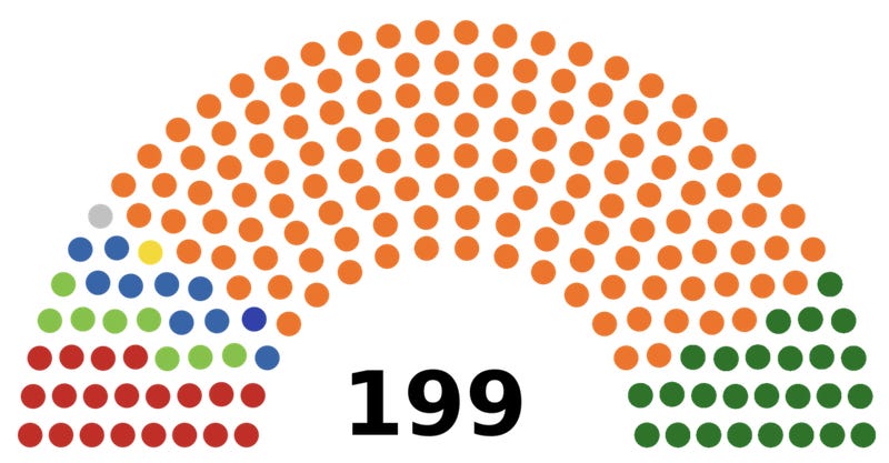
Thirdly, there is the issue of the margin of error. We never find perfectly proportional results, but we have to interpret the numbers somehow. We can make statements in an ordinal fashion, like: the 2014 election in Hungary (pictured below) resulted in the most disproportionate parliament since 1989 according to the Gallagher index. But is there something that we call ‘proportional’, or was everything just disproportionate to different degrees? For the Loosemore-Hanby and Gallagher indices, a result of about 5(%) or below is the rule of thumb for calling a result proportional. For the former, this means 5% of ‘wasted votes’, but for the latter, we may want to insist on benchmark lower than 5%.
Recommended (academic) reading on this subject:
Taagepera, R. and Grofman, B., 2003. Mapping the indices of seats–votes disproportionality and inter-election volatility. Party Politics, 9(6), pp.659-677.
Gallagher, M., 1991. Proportionality, disproportionality and electoral systems. Electoral Studies, 10(1), pp.33-51.
Cox, G.W. and Shugart, M.S., 1991. Comment on Gallagher’s ‘proportionality, disproportionality and electoral systems’. Electoral Studies, 10(4), pp.348-352.